AI Academic Notes

Concepts

TP, TN, FP, FN

TP: true positive, meaning that the prediction is "positive" and it is true.

TN: true negative, the prediction is "negative" and it is true.

FP: false positive, the prediction is "positive" and it is false (the correct answer is "negative").

FN: false negative, meaning that the prediction is "negative" and it is false (the correct answer is "positive").

Dice loss

Dice loss is widely used in sematic segmentation, e.g. in medical image segmentation tasks, to address the data imbalance problem.

The Dice coefficient (or Dice similarity coefficient) :

The Dice loss:

In the case of multi-class Dice loss, the Intersection and Union calculation is done over each class and the result is averaged to obtain the final Dice loss value. The lower the Dice loss value, the better the segmentation results.

Also see Common Loss Functions: Dice Loss.

Soft K-means

Soft K-means is an extension of K-means algorithm where instead of assigning each data point to a cluster with hard assignment, each data point is assigned a probability of belonging to each cluster. This allows a data point to belong to multiple clusters with different degrees of membership, whereas in K-means, a data point can only belong to one cluster.

In soft K-means, a data point is assigned a membership value for each cluster based on its similarity to the cluster centroid. The membership values are represented as probabilities, and each data point is assigned to the cluster with the highest probability. Soft K-means is useful when the boundaries between clusters are not well-defined, or when a data point can belong to multiple clusters.

EM algorithm

The Expectation-Maximization (EM) algorithm is an iterative optimization algorithm used to estimate the parameters of statistical models, particularly those with latent variables.

The EM algorithm is a two-step process. In the first step (the expectation or E-step), the algorithm estimates the expected value of the log-likelihood function using the current estimates of the parameters. In the second step (the maximization or M-step), the algorithm maximizes this expected log-likelihood function with respect to the parameters. The process is repeated until convergence is reached and the estimates of the parameters stabilize.

The EM algorithm is widely used in machine learning and data analysis for tasks such as clustering, classification, and density estimation.

Log-likelihood function

We use the log-likelihood function because it has several mathematical properties that make it easier to work with than the regular likelihood function. Some of these properties include:

1. Logarithms convert products to sums: Since likelihoods of individual data points are typically multiplied together to form the overall likelihood, taking the logarithm of the likelihood turns the multiplication into a summation, which is easier to work with mathematically.

   When calculating the joint probability of an independent and identically distributed dataset, like

   $$X=\left\{x_{1}, x_{2}, \ldots, x_{N}\right\}$$

   the joint probability is

   $$p(X \mid \Theta)=\prod_{i=1}^{N} p\left(x_{i} \mid \Theta\right)$$

   Taking logarithms on both sides can turn the multiplication into a summation.

   $$\ln p(X \mid \Theta)=\sum_{i=1}^{N} \ln p\left(x_{i} \mid \Theta\right)$$

2. Logarithms are monotonically increasing: This means that if we have two models that we want to compare, we can compare their log-likelihoods instead of their likelihoods, and the result will be the same.

   $$p\left(x \mid \Theta_{1}\right)>p\left(x \mid \Theta_{2}\right) \Leftrightarrow \ln p\left(x \mid \Theta_{1}\right)>\ln p\left(x \mid \Theta_{2}\right)$$

3. Log-likelihood is more numerically stable: Computing likelihoods of data points involves multiplying many probabilities together, which can lead to numerical instability. Taking the logarithm of the likelihoods can help avoid issues with floating point arithmetic and numerical precision (e.g., we can avoid issues with underflow when dealing with very small likelihood values). Note: Underflow occurs when the values are too small to be represented by the floating-point precision of the computer.

Transductive learning and inductive learning

• Transductive learning: take-home exam. The goal of transductive learning is to transduce information from labeled training datasets to available unlabeled (training) data.
• Inductive learning: in-class exam. The goal of inductive learning is to generalize to new data. Thus, inductive learning refers to building a learning algorithm that learns from a labeled training set and generalizes to new data.

Transductive learning refers to a type of machine learning that involves predicting the labels of unlabeled data points in a given dataset, which means that the train dataset (labeled) and the test dataset (unlabeled) are both available when learning, thereby sometimes being considered as one dataset. The goal of transductive learning is to improve the accuracy of the predictions for the labeled data points and the unlabeled data points that are part of the same dataset.

In transductive learning, the model learns to predict outputs for specific unlabeled data points based on their proximity to labeled data points in the training set. However, the model does not learn a general mapping from inputs to outputs that can be applied to new, unseen data points. This is because transductive learning only makes predictions for specific instances that were available during training, rather than learning a general pattern that can be applied to any new input.

Transduction (transductive inference) is a related concept to transductive learning, but they are not exactly the same thing. Transduction was introduced by Vladimir Vapnik (who is also the creator of SVM) in the 1990s.

Transductive inference is a general concept in computer science and machine learning that refers to the process of making predictions for specific, individual examples, based on knowledge or observations of other, related examples. In other words, transductive inference involves predicting the output of a specific example based on the input and output of other examples that are similar or related to it.

So, we can see that transduction or transductive inference is a process of reasoning, but transductive learning is a process of learning. That is, we can view transductive learning as an algorithm or one of the algorithms for achieving transductive inference. So is the relationship between induction (inductive inference) and inductive learning.

Transduction vs Induction

Transduction is reasoning from observed, specific (training) cases to specific (test) cases. In contrast, induction is reasoning from observed training cases to general rules, which are then applied to the test cases.

Inductive learning is the same as what we commonly know as traditional supervised learning?

Yes, that's correct. Inductive semi-supervised learning is a type of inductive learning, which is commonly known as supervised learning. In inductive semi-supervised learning, the algorithm learns a function that maps inputs to outputs using a labeled training set, and then applies that function to new, unseen data points to make predictions. The difference between inductive supervised learning and inductive semi-supervised learning is that in the latter, the algorithm also has access to some unlabeled data during training, which can improve its performance.

(see Semi-supervised learning).

(There is another type of semi-supervised learning called "inductive semi-supervised learning," which aims to learn a general mapping from inputs to outputs that can be applied to new, unseen data points. In this approach, the model is trained on both labeled and unlabeled data and aims to learn a general pattern that can be used to predict outputs for any new input. Inductive semi-supervised learning is more challenging than transductive learning because it requires the model to generalize beyond the specific instances available during training.)

Supplementary Notes:

"inductive" vs "deductive", see the picture below.

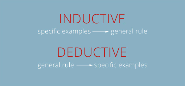
(image source: https://www.netlanguages.com/blog/wp-content/uploads/2017/06/diagram.jpg)

Note: I think Transductive learning and Inductive learning are rarely mentioned, maybe their difference is not obvious enough, or this difference is downplayed?

SVM and TSVM

Support Vector Machines (SVMs) are supervised learning models for a problem where we try to find a hyperplane that best separates the two classes.

1. Linear SVM

   When the data is perfectly linearly separable only then we can use Linear SVM. Perfectly linearly separable means that the data points can be classified into 2 classes by using a single straight line(if 2D).

2. Non-Linear SVM

   When the data is not linearly separable then we can use Non-Linear SVM, which means when the data points cannot be separated into 2 classes by using a straight line (if 2D) then we use some advanced techniques like kernel tricks to classify them. In most real-world applications we do not find linearly separable data points hence we use "kernel trick" (introduced later) to solve them.

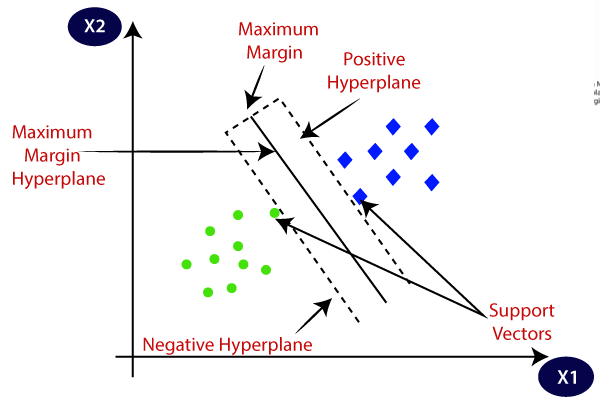
(image source: https://editor.analyticsvidhya.com/uploads/567891.png)

Margin is a important concept in SVM, which is the distance between the hyperplane and the observations closest to the hyperplane (support vectors). In SVM, a large margin is considered a good margin. There are two types of margins: the hard margin and the soft margin.

In SVMs, the goal is to find the hyperplane that best separates the data into different classes. In the case of linearly separable data, a hard margin SVM seeks to find the hyperplane that separates the classes with a margin that is as large as possible.

A soft margin SVM allows for some points to be on the wrong side of the margin or even misclassified. The soft margin SVM balances the desire for a large margin with the need to allow some misclassification, and includes a tuning parameter, called the regularization parameter, which controls the trade-off between these two goals. We can use SVM Error = Margin Error + Classification Error to evaluate the objective, where the higher the margin, the lower would-be margin error, and vice versa.

We need "kernel tricks" to make it easier for SVM to work with a non-linear dataset. The function of kernel is to take data as input and transform it into the required form (e.g., converting a lower dimension space to a higher dimension space, mapping the inputs to a value of 0 or 1). Finally, the kernel trick avoids the explicit mapping that is needed to get linear learning algorithms to learn a nonlinear function or decision boundary. Examples of kernels: polynomial kernel, sigmoid kernel, radial basis function (RBF) kernel.

The choice of kernel for SVM can have a significant impact on its performance. SVM with a well-chosen kernel can be very effective in a wide range of classification and regression problems. However, choosing an appropriate kernel can be challenging (kernels are where the nonlinearity is the introduced in the SVM algorithm), as different kernels have different strengths and weaknesses and may be better suited for different types of data and classification problems. Additionally, kernel selection often involves a trade-off between model complexity and performance, and it is typically based on trial and error, domain knowledge, or optimization techniques.

Transductive Support Vector Machine (TSVM) is a variant of Support Vector Machine (SVM) that can be used for semi-supervised learning tasks (see Semi-supervised learning). TSVM is designed to work with partially labeled data, where only a small portion of the data is labeled, and the majority of the data is unlabeled.

TSVM uses both labeled and unlabeled data in the training phase, whereas standard SVM only uses labeled data. This makes TSVM a semi-supervised learning method (see Semi-supervised learning), while standard SVM is a supervised learning method. Additionally, TSVM is designed specifically for transductive learning (see Transductive learning and inductive learning), where we aim to predict the labels of specific, known test points, while standard SVM is more general and can be used for any kind of supervised learning task.

The TSVM algorithm iteratively assigns labels to the unlabeled data points, based on their proximity to the decision boundary, and re-estimates the boundary based on the newly labeled points. This process continues until a stable decision boundary is reached. TSVM algorithm needs to be executed iteratively because the labels assigned to the unlabeled data points affect the decision boundary of the SVM. As more unlabeled data points are assigned labels, the decision boundary may change, and the previously labeled data points may be relabeled.

Semi-supervised learning

What is Semi-supervised learning (SSL)?

• Supervised learning + Additional unlabeled data
• Unsupervised learning + Additional labeled data

Semi-supervised learning is a special case of weakly supervised learning. It falls in between supervised and unsupervised learning. We can conduct semi-supervised learning as either inductive or transductive learning, and both may be performed using a semi-supervised learning algorithm.

First-order and second-order moments

In optimization algorithms, first-order and second-order moments are often used to guide parameter updates. These moments are calculated from historical gradients and help improve the optimization process.

1. First-order moment: The first-order moment can be thought of as an exponentially weighted moving average of historical gradients. The first-order moment captures the direction of the gradient and can improve the stability and speed of the optimization process. This is commonly used in momentum-based optimization methods and the Adam optimizer.
2. Second-order moment: The second-order moment is the exponentially weighted moving average of the squared historical gradients. The second-order moment captures the magnitude information of the gradient. In the optimization process, the second-order moment helps to adaptively adjust the learning rate, applying different update sizes on different parameters. The second-order moment is commonly used in AdaGrad, RMSProp, and Adam optimizers.

In practice, combining first-order and second-order moments can improve the optimization process. For example, the Adam optimizer combines both the first-order and second-order moments to achieve adaptive learning rate adjustment and better optimization results.

$L_1$, $L_2$, $L_p$, $L_∞$ norms and regularizations

What is Norm?

In simple words, the norm is a quantity that describes the size of a vector, something that we can represent using a set of numbers as you might already know that in machine learning everything is represented in terms of vectors. In this norm, all the components of the vector are weighted equally.

$L_0$ norm

It is actually not a norm (See the conditions a norm must satisfy here; L0 norm doesn't satisfy the absolute homogeneity). Corresponds to the total number of nonzero elements in a vector. For example, the L0 norm of the vectors (0,0) and (0,2) is 1 because there is only one nonzero element.

L0 norm is computationally hard and prone to overfitting. People use the L1 norm as a preferred choice in practice because it is easier to optimize and promotes sparsity effectively.

$L_1$ norm (Taxicab norm or Manhattan norm; derived distance: Manhattan distance)

$\|\boldsymbol{x}\|_{1} := \sum_{i=1}^n |x_i|$

$L_2$ norm (Euclidean norm; derived distance: Euclidean distance)

$\|\boldsymbol{x}\|_{2} := \sqrt{\sum_{i=1}^n x_i^2}$

$L_p$ norm (p-norm)

$\|\boldsymbol{x}\|_{p} := \left(\sum_{i=1}^n |x_i|^p\right)^{\frac{1}{p}}$

$L_∞$ norm (maximum norm, uniform norm, or supremum norm)

$\|\boldsymbol{x}\|_{\infty}:=\lim\limits_{p \mapsto \infty}\left(\sum_{i=1}^{n}\left|x_{i}\right|^{p}\right)^{\frac{1}{p}}$

$\|\boldsymbol{x}\|_{\infty}:=\max _{1 \leq j \leq n}\left\{\left|x_{1}\right|, \left|x_{2}\right|, \ldots, \left|x_{n}\right|\right\}$

$L_{\infty}$ measures the maximum absolute value of a vector component. The set of vectors whose infinity norm is a given constant, $c$, forms the surface of a hypercube with edge length $2c$.

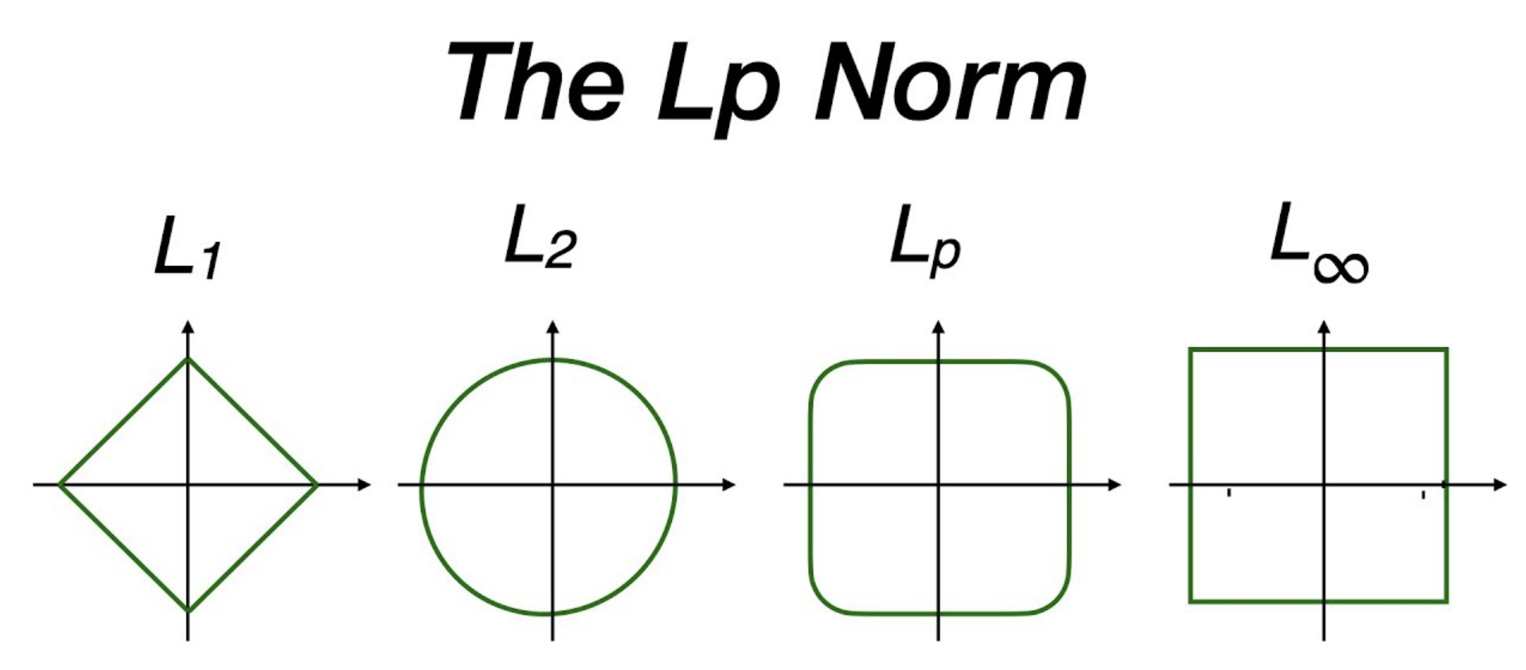
$L_1$ regularization (Lasso regression)

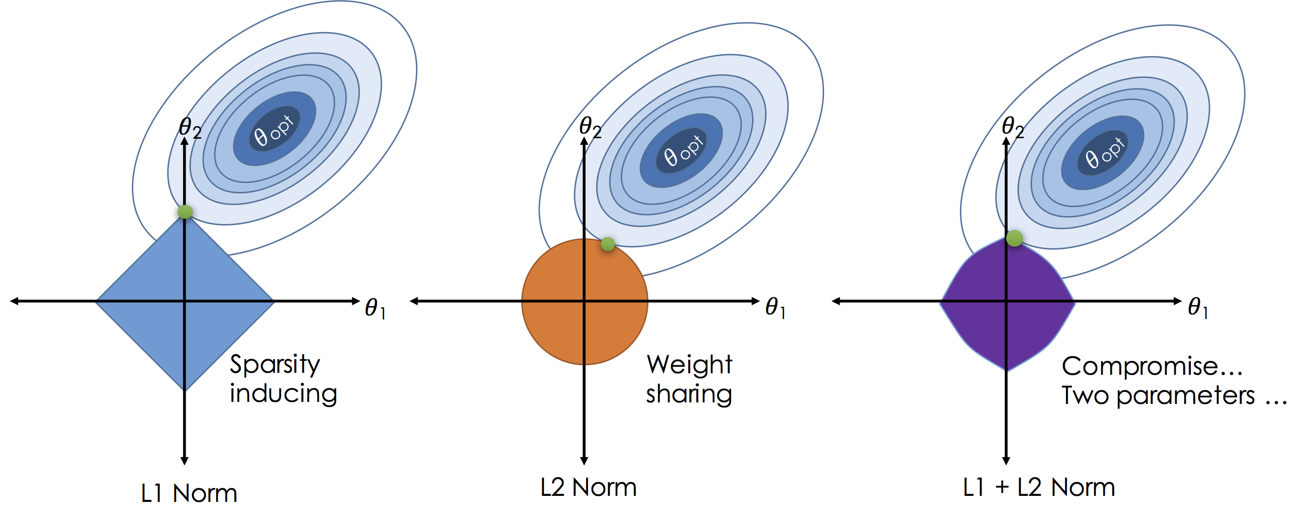
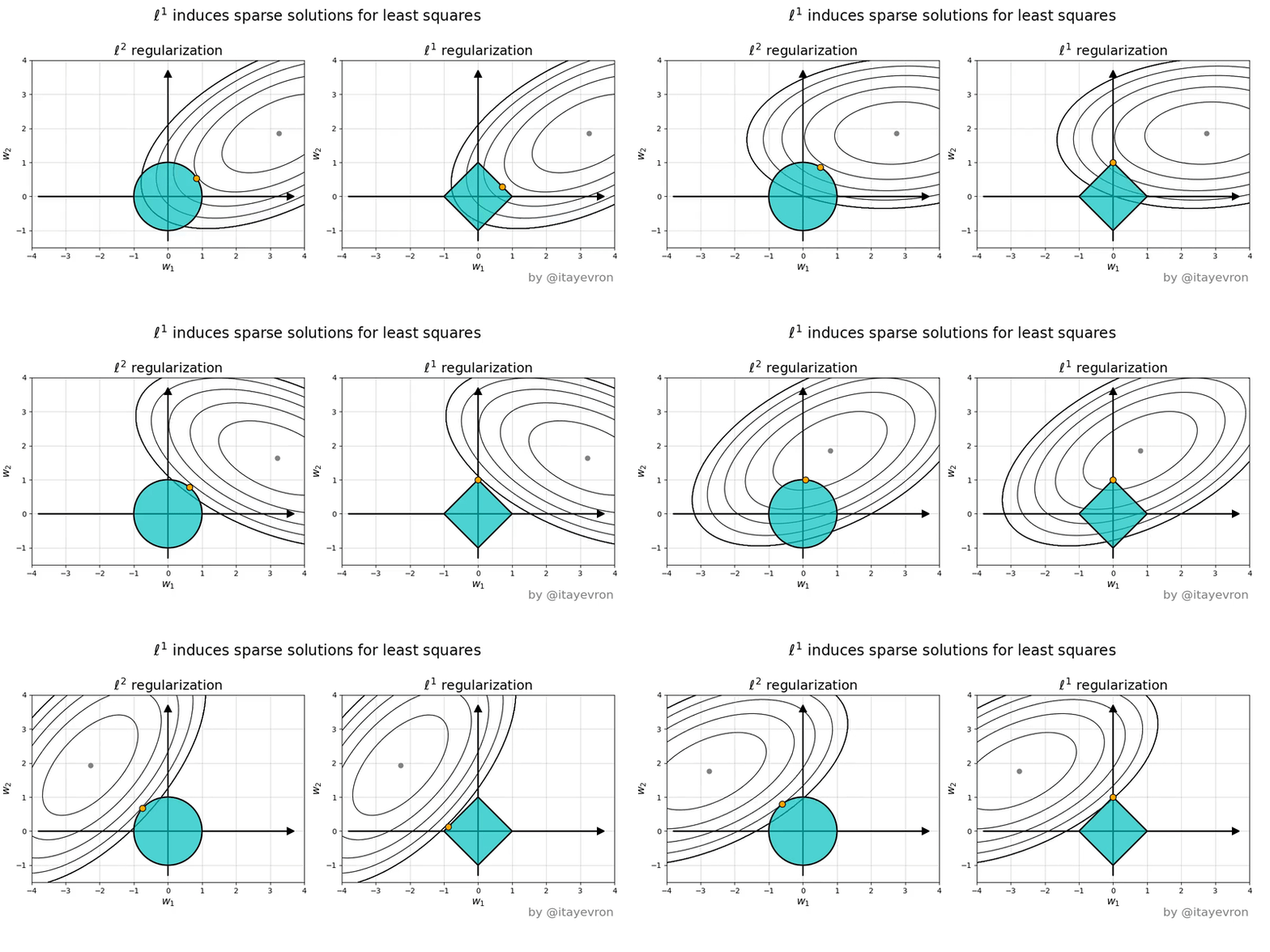
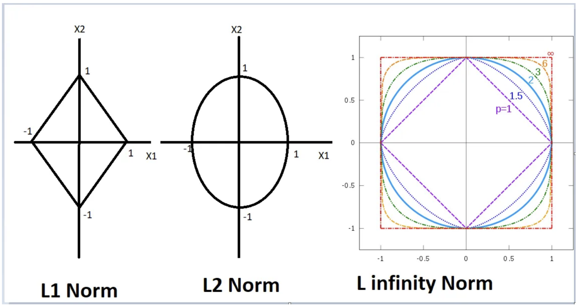
L1 regularization adds the sum of the absolute values of the weights (parameters) of the model to the loss function. The L1 regularization term encourages sparsity by driving some of the weights to become exactly zero -- this happens because the L1 norm has "sharp corners" at zero (see pictures). This property makes L1 regularization useful for feature selection, as it indicates which features are more important. See pictures below for why using $L_1$ norm shape to touch the solution surface will very likely to find a touch point on a spike tip and thus a sparse solution.

The term "lasso" in Lasso Regression is an acronym for "Least Absolute Shrinkage and Selection Operator."

$L_2$ regularization (ridge regression)

L2 regularization adds the sum of the squared values of the weights to the loss function. The L2 regularization term encourages smaller weight values without driving them to zero. It penalizes large weights more strongly than L1 regularization and helps prevent overfitting by discouraging the model from relying too heavily on any single feature. The L2 regularization term promotes smoothness in the weight values and can improve the model's robustness to noise in the training data. See the pictures below to compare $L_1$ and $L_2$ regularizations.

The term "ridge" in Ridge Regression reflects the geometric interpretation of the regularization term, which shapes the error surface into a ridge-like structure and encourages the weights to be more evenly spread out.

$L_∞$ regularization (max norm regularization)

$L_∞$ regularization encourages stability and robustness by preventing any individual coefficient from becoming too large. This helps to control the impact of individual parameters and promotes stability in the model. It is useful when there is a need to restrict extreme parameter values and prevent them from dominating the model's behavior.

The figures below are the geometric perspective on sparsity and the $L_1$ norm and $L_2$ norm.

Views